
Can Machine Learning of Magnetic Resonance Imaging Textural Features Differentiate Intra- and Extra-Axial Brain Tumours? A Feasibility Study
ORIGINAL ARTICLE
Hong Kong J Radiol 2025;28:Epub 12 September 2025
Can Machine Learning of Magnetic Resonance Imaging Textural Features Differentiate Intra- and Extra-Axial Brain Tumours? A
Feasibility Study
Ohoud Alaslani1, Nima Omid-Fard1, Rebecca Thornhill1, Nick James2, Rafael Glikstein1
1 Department of Radiology, University of Ottawa, Ottawa, Canada
2 Systems Integration and Architecture, The Ottawa Hospital, Ottawa, Canada
Correspondence: Dr R Glikstein, Department of Radiology, University of Ottawa, Ottawa, Canada. Email: rglikstein@toh.ca
Submitted: 4 January 2024; Accepted: 3 September 2024. This version may differ from the final version when published in an issue.
Contributors: OA, RT, NJ and RG designed the study. OA, RT and NJ acquired the data. All authors analysed the data. OA, NO, RT and NJ
drafted the manuscript. All authors critically revised the manuscript for important intellectual content. All authors had full access to the data,
contributed to the study, approved the final version for publication, and take responsibility for its accuracy and integrity.
Conflicts of Interest: All authors have disclosed no conflicts of interest.
Funding/Support: This research received no specific grant from any funding agency in the public, commercial, or not-for-profit sectors.
Data Availability: All data generated or analysed during the present study are available from the corresponding author on reasonable request.
Ethics Approval: This research was approved by Ottawa Health Science Network Research Ethics Board, Canada (Ref No.: #2020033-01H). A waiver of patient consent was granted by the Board due to the retrospective nature of the research.
Abstract
Introduction
Determining the origin of intracranial lesions can be challenging. This study aimed to assess the
feasibility of a machine learning model in distinguishing intra-axial (IA) from extra-axial (EA) brain tumours using
magnetic resonance imaging (MRI).
Methods
We retrospectively reviewed 92 consecutive adult patients (age >18 years) with newly diagnosed solitary brain lesions who underwent contrast-enhanced brain MRI at our institution from January 2017 to December 2018. Tumour volumes of interest (VOIs) were manually segmented on both T2-weighted (T2W) and T1-weighted (T1W) post-contrast images. An XGBoost machine learning algorithm was used to generate classification models based on textural features extracted from the segmented VOIs, with histopathology as the reference standard.
Results
Among the 92 lesions analysed, 70 were IA and 22 were EA. The area under the receiver operating characteristic curve for identifying IA tumours was 0.91 (95% confidence interval [95% CI] = 0.89-0.93) for the T1W post-contrast model, 0.81 (95% CI = 0.78-0.84) based on T2WI model, and 0.92 (95% CI = 0.90-0.94) for the combined model. All models demonstrated high sensitivity (>90%) for identifying intra-axial tumours, though specificity was lower (39%-64%). Despite this, models achieved acceptable levels of accuracy (>80%) and precision (>88%).
Conclusion
This preliminary study demonstrates the feasibility of a machine learning classification model for
differentiating IA from EA tumours using MRI textual features. While sensitivity was high, specificity was limited,
likely due to the class imbalance. Further studies with balanced datasets and external validation are warranted.
Key Words: Machine learning; Magnetic resonance imaging; Neoplasms
中文摘要
磁力共振影像紋理特徵的機器學習能否區分腦內與腦外腫瘤?一項可行性研究
Ohoud Alaslani, Nima Omid-Fard, Rebecca Thornhill, Nick James, Rafael Glikstein
引言
確定顱內病變的來源可具挑戰性。本研究旨在評估機器學習模型在磁力共振影像中區分腦內與腦外腫瘤的可行性。
方法
本研究回顧分析2017年1月至2018年12月期間於本院接受增強磁力共振影像檢查的92位連續成年患者(年齡18歲以上),這些患者均為新診斷的單發性腦病變個案。研究人員於T2加權影像及T1加權增強影像上手動分割腫瘤感興趣體積,並從中提取紋理特徵。之後,應用XGBoost機器學習演算法,並以組織病理學結果為參考標準,建立分類模型。
結果
92個病灶中,70個為腦內腫瘤,22個為腦外腫瘤。T1加權增強影像模型辨識腦內腫瘤的受試者工作特徵曲線下面積為0.91(95%置信區間 = 0.89-0.93),T2加權影像模型為0.81(95%置信區間 = 0.78-0.84),組合模型則為0.92(95%置信區間 = 0.90-0.94)。所有模型對識別腦內腫瘤均表現出較高敏感度(>90%),但特異性相對較低(39%-64%)。儘管如此,模型仍達到了可接受的準確度(>80%)與精確度(>88%)。
結論
本初步研究證實,應用磁力共振影像紋理特徵建立機器學習分類模型,有助於區分腦內與腦外腫瘤。雖然模型具備良好敏感度,但特異性較低,可能與類別不平衡有關。建議未來研究採用類別平衡的資料集,並進行外部驗證,以提升模型效能與泛化能力。
INTRODUCTION
Intracranial tumours can pose a diagnostic challenge
in clinical practice. Recent advancements in artificial
intelligence in radiology may provide additional
diagnostic information. Radiomics techniques such as
texture analysis can reveal grey-level patterns beyond
what is possible through expert human visual perception
alone.[1] Numerous quantitative textural features can be
derived, including simple statistics based on grey-level
histograms, and higher-order features based on spatial
relationships among pixels.[2] These radiomic features,
derived from conventional magnetic resonance imaging
(MRI) sequences, can be leveraged to train various
machine learning (ML) models to detect and classify
brain tumours, as well as predict prognosis and treatment
response.[3] [4] [5]
Previous applications of radiomics in brain tumour
research have aimed to improve diagnosis and
post-treatment imaging of gliomas, including
grading, distinguishing tumour progression from
pseudoprogression, patient survival, and genetic expression.[3] [4] Other neuro-oncologic ML advances
include differentiating gliomas from mimics such
as meningiomas, pituitary tumours, and solitary
metastases,[5] [6] diagnosis of paediatric tumours,[7] [8] and
detecting metastases.[9] Radiomic approaches can offer more consistent results with good external validity,
compared to the interrater variability of human readers.[6]
More recently, deep learning models trained to detect
brain metastases have shown advantages over classical
ML in terms of lower false-positive rates albeit with
greater training data requirements.[9]
Accurately determining whether a lesion arises from
within the brain parenchyma (intra-axial, IA) or from
the surrounding structures (extra-axial, EA) is crucial
for diagnosis and treatment planning. This study aimed
to determine whether ML of MRI radiomic features can
differentiate between IA and EA locations.
METHODS
Patient Population
This retrospective study performed at a single tertiary-care academic centre. Medical record review was
conducted per the guidelines of the Institutional Review
Board. We identified 92 consecutive adult patients
(age >18 years) who underwent brain MRI for a newly
diagnosed solitary brain lesion from January 2017 to
December 2018. Patients with multiple lesions or prior
surgery or chemo/radiotherapy were excluded. Data on
age, sex, and final histopathology were recorded.
Magnetic Resonance Imaging
MRI of the brain was performed using 1.5 T (25 IA and
9 EA tumours; Siemens Magnetom Symphony, Siemens
Medical Systems, Erlangen, Germany) or 3 T (45 IA and
13 EA tumours; Siemens Tim Trio or GE DISCOVERY
MR 750w, GE Medical Systems, Milwaukee [WI], US)
systems. Using a dedicated head coil, three-dimensional
(3D) axial stacks of T1-weighted (T1WI) post-contrast
and T2-weighted images (T2WI) were acquired with
the following parameters: 1.5 T: T2WI (fast spin echo
with fat saturation): TR/TE 3510/97, echo train length
9, flip angle 180°, section thickness 5.5 mm; T1W post-contrast
(fast spoiled gradient echo with fat saturation):
TR/TE 6.73/2.71, flip angle 15°, section thickness 1 mm.
3 T: T2WI (fast spin echo with fat saturation): TR/TE
6700/97, echo train length 18, flip angle 120°, section
thickness 3 mm; T1WI post-contrast (fast spoiled gradient
echo): TR/TE 8.48/3.21, flip angle 12°, section thickness
1 mm. Post-contrast T1WI images were acquired after
hand injection of 0.1 mmol/kg of gadobutrol (Gadovist;
Bayer Healthcare, Hong Kong, China), followed by a
10-20 mL saline flush, using a 4–5-minute delay before
acquisition at 3 T and a 6-to-7-minute delay at 1.5 T.
All images were reviewed using a Picture Archiving Computed System (PACS; Horizon Medical Imaging,
McKesson Corporation, San Francisco [CA], US).
Histopathology
The IA or EA designation was confirmed by final
histopathology following biopsy, extracted from
the electronic medical records. The specimens were
obtained by the neurosurgeons and analysed by the
neuropathologists at our centre.
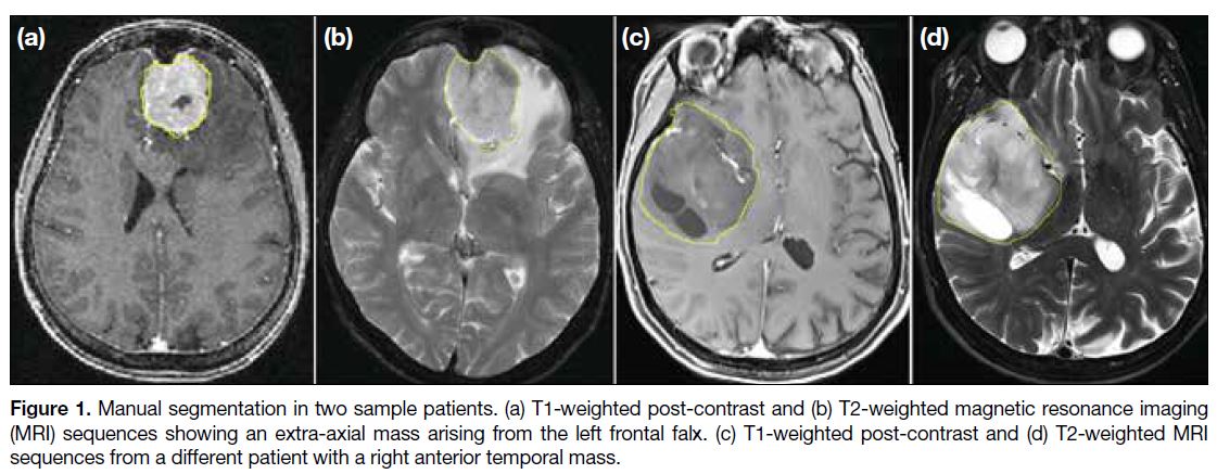
Image Analysis and Tumour Segmentation
Tumour volumes of interest (VOI) were manually
segmented on both T2WI and post-contrast T1WI using
ImageJ version 1.52r (National Institutes of Health, US,
https://imagej.net/) by a neuroradiology fellow, under
supervision of a staff neuroradiologist with over 30 years
of experience. VOI contours were subsequently submitted
to a blinded medical imaging scientist (redacted/blinded
for review) for texture analysis. Examples are shown in
Figure 1.
Figure 1. Manual segmentation in two sample patients. (a) T1-weighted post-contrast and (b) T2-weighted magnetic resonance imaging (MRI) sequences showing an extra-axial mass arising from the left frontal falx. (c) T1-weighted post-contrast and (d) T2-weighted MRI sequences from a different patient with a right anterior temporal mass.
First- and second-order statistical textural features
were computed for each VOI and MRI sequence using
MaZda software (version 4.6.0; Institute of Electronics,
Technical University of Lodz, Lodz, Poland).[10] First-order
features included grey-level histogram mean,
variance, skewness, kurtosis, and percentile values (1st
to 99th). Second-order features included grey-level
co-occurrence matrix (GLCM[11]) and run-length matrix
(RLM[12]) features (11 GLCM and 5 RLM features per
sequence) Before computing GLCM and RLM features,
signal intensities were normalised between μ ± 3σ
(where μ was the mean value of grey levels inside the VOI [or VOI subzone] and σ was the standard deviation)
and decimated to 32 grey levels to minimise inter-scanner
variability.[13] [14]
Machine Learning and Classification
We used XGBoost,[15] an open-source ML algorithm,
to train models on the textural features extracted from
T2WI, T1WI post-contrast, and their combination.
Hyperparameters were tuned using an 100-trial Bayesian
optimisation experiment via GPyOpt[16] (http://github.com/SheffieldML/GPyOpt), guided by Gaussian process
modelling and an exploration-exploitation heuristic. Each model was evaluated using stratified ten-fold cross-validation, repeated 10 times.[17] The SHAP (Shapley Additive exPlanations) framework[18] was used to estimate each feature’s relative importance, normalised to sum to 1.0.
Statistical Analysis
Statistical analysis was performed using RStudio, an
open-source software (version 1.3.1093; PBC, Boston
[MA], US). Mann-Whitney U tests were used to
compare IA and EA groups for each feature. Stepwise
Holm-Bonferroni correction was applied for multiple
comparisons.[19] Model performance was assessed
using accuracy, the area under the receiver operating
characteristic curve (AUC), sensitivity, specificity,
precision, and F1 score. ROC confidence intervals
(95% CI) were calculated using 5000 bootstrap iterations,
and AUC differences were assessed using DeLong’s
method.[20]
RESULTS
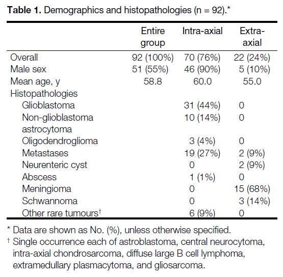
A total of 92 lesions were analysed (70 IA and 22 EA).
Table 1 summarises demographics and histopathological
data. Glioblastomas (44%) and metastases (27%) were
the most common diagnoses in the IA group, while
meningiomas (68%) were the most common in the EA
group. The patients aged from 23 to 84 years, with a
mean age of 58.8 years. No significant difference was
noted between groups (IA median, 62 years [interquartile
range, 18] vs. EA median, 55 years [interquartile range,
10]; p = 0.09). Males were more common in the IA group
(66% vs. 23%; p < 0.01).
Table 1. Demographics and histopathologies (n = 92).
Radiomic Features
Table 2 provides median and interquartile range values
for individual 3D textural features. EA tumours showed
higher histogram mean, kurtosis, and 10th and 50th
percentiles on T1WI post-contrast, and lower skewness
(p < 0.001 for all). On T2WI, only kurtosis was
significantly higher in the EA group (p < 0.001), while
the 90th and 99th percentiles were significantly lower
(p = 0.002 and 0.001, respectively).
Table 2. Median values of 25 individual textural features used in machine learning classification.
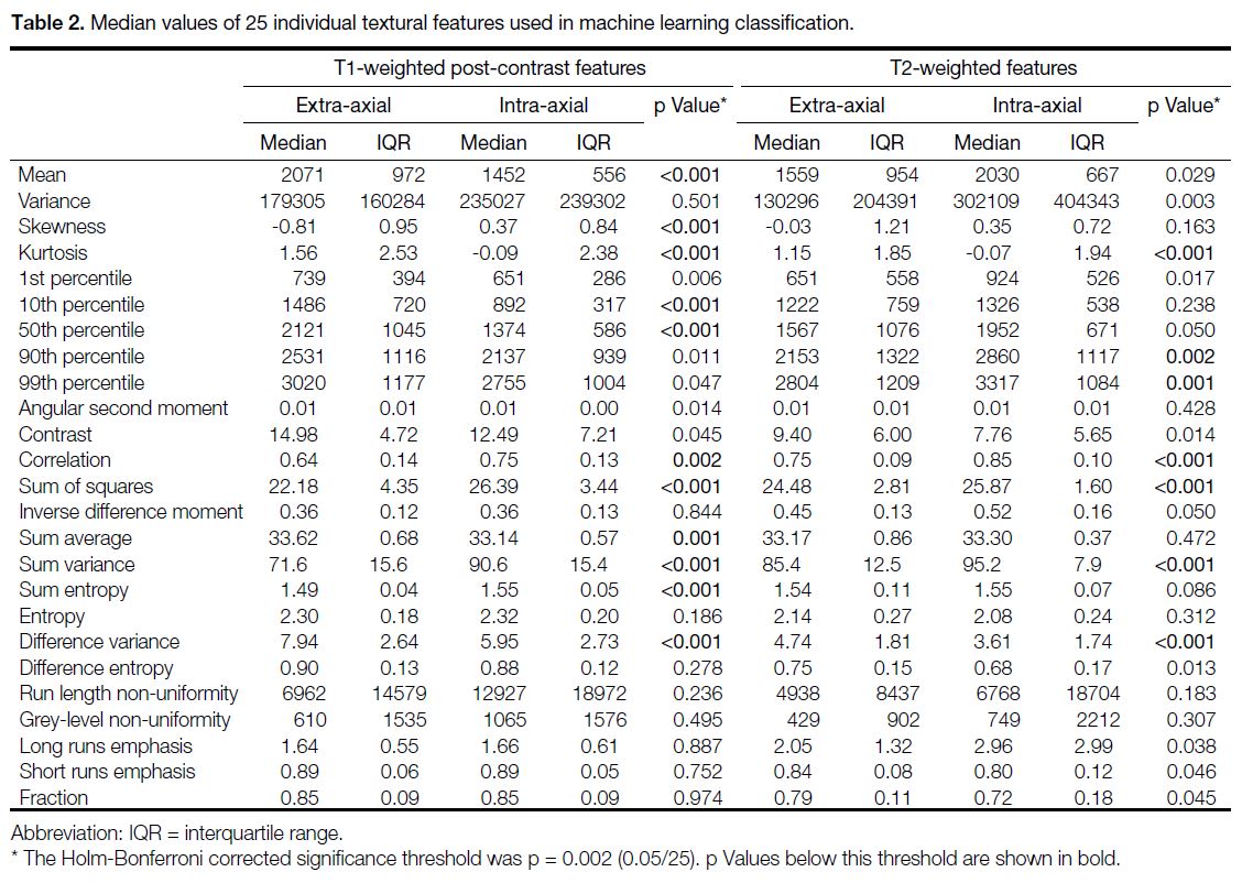
Among the second-order features computed from T1W
post-contrast images, GLCM correlation, sum of squares,
sum variance, and sum entropy associated with EA
tumours were significantly lower than those computed
for the IA group (p = 0.002 for correlation and p < 0.001
for the rest; Table 2). The T1 GLCM sum average and
difference variance were both significantly greater in
EA tumours compared to the IA group (p = 0.001 and
p < 0.001, respectively). Similar to T1 post-contrast, the
GLCM correlation, sum of squares, and sum variance
features evaluated from T2 images were significantly
lower than those in the IA group (p < 0.001 for each).
The T2 GLCM difference variance was significantly
greater in EA tumours compared to the IA group
(p < 0.001). Among the group differences assessed for
RLM features, none was found to be significant after
Holm–Bonferroni correction for multiple comparisons
(Table 2).
The classification performance metrics for each of the
three ML models are summarised in Table 3. Receiver
operating characteristic curves and feature attribution
scores are depicted in Figures 2, 3, and 4. The AUC for the
identification of IA tumours was 0.91 (95% CI = 0.89-0.93; Figure 2a) for the model based on T1-weighted
post-contrast MRI features, 0.81 (95% CI = 0.78-0.84;
Figure 3a) based on T2-weighted MRI features, and 0.92 (95% CI = 0.90-0.94; Figure 4a) based on all features.
Table 3. Classification performance metrics for each magnetic resonance imaging textural feature of the machine learning
model.
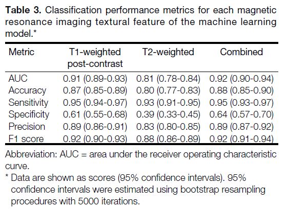
Figure 2. (a) Receiver operating characteristic curve showing the area under the curve (AUC) for the XGBoost model, and (b) SHAP (Shapley
Additive exPlanations) feature importance plot for the same model trained on T1-weighted post-contrast magnetic resonance imaging
textural features to identify intra-axial tumours. SHAP values are aggregated across samples and normalised to sum to 1.0.
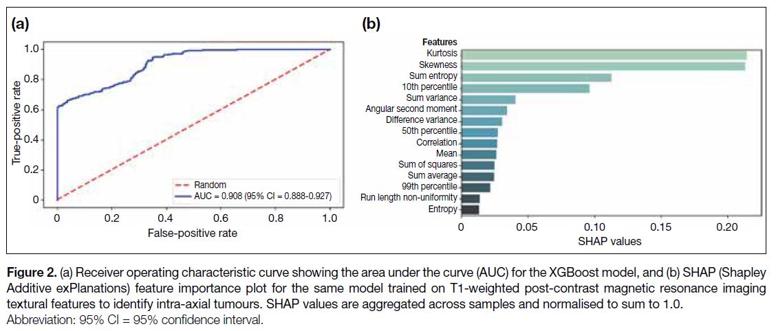
Figure 3. (a) Receiver operating characteristic curve showing the area under the curve (AUC) for the XGBoost model, and (b) SHAP (Shapley
Additive exPlanations) feature importance plot for the same model trained on T2-weighted magnetic resonance imaging textural features to
identify intra-axial tumours. SHAP values are aggregated across samples and normalised to sum to 1.0.
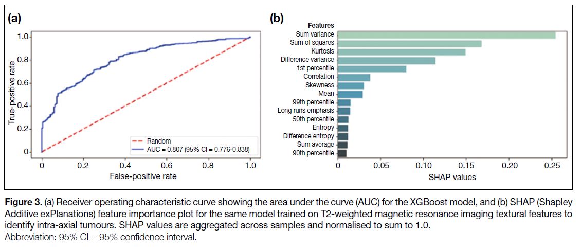
Figure 4. (a) Receiver operating characteristic curve showing the area under the curve (AUC) for the XGBoost model, and (b) SHAP (Shapley
Additive exPlanations) feature importance plot for the same model trained on combined T1-weighted post-contrast and T2-weighted
magnetic resonance imaging textural features to identify intra-axial tumours. SHAP values are aggregated across samples and normalised
to sum to 1.0.
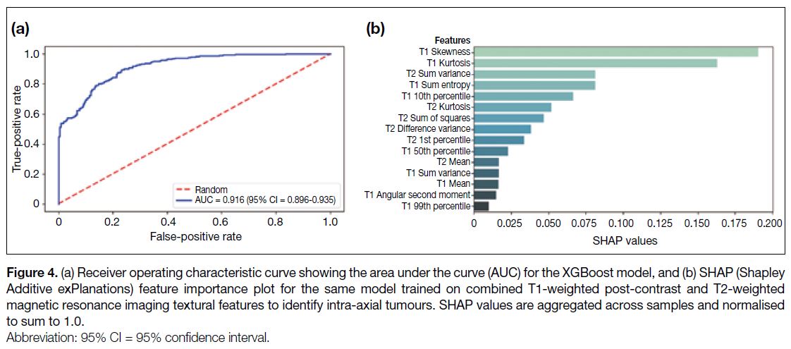
Table 3 shows that the three models (T1WI, T2WI, and
combined) yielded AUCs that were significantly greater
than 0.5 (p < 0.0001 for each comparison). The model
produced by the T2WI features alone resulted in an AUC that was significantly lower than the model produced by
either the T1W post-contrast or combined sequences
(p < 0.0001 for each comparison). The combined model
AUC was not significantly greater than the T1 model alone (p = 0.135). All models had high sensitivity in
identifying intra-axial tumours (>90% for each), but none
achieved high specificity (39%-64%). Nevertheless, the
models attained acceptable levels of accuracy (>80%)
and precision (>88%).
The feature importance attribution profile associated
with the model trained using T1W post-contrast MRI
features reveals that grey-level kurtosis, skewness,
sum entropy, 10th (histogram) percentile, and sum
variance contributed two thirds of the total proportional
importance score (0.67/1.00) for this model (Figure 2b).
Sum variance and kurtosis also contributed strongly towards the total proportional importance of the T2-based model (0.40/1.00), with sum of squares, difference
variance, and 1st percentile contributing an additional
0.36/1.00 towards the total proportional importance for
the T2-based model (Figure 3b). In the combined model,
the T1WI skewness, kurtosis, sum entropy, and 10th
percentile were found to represent four of the five ‘most
important’ features, contributing 0.50/1.00 of the total
proportional importance (Figure 4b).
DISCUSSION
Classically described features of EA lesions include
broad-based dural attachment, adjacent bony changes,
formation of a cerebrospinal fluid cleft, deviation of pial
vessels, and buckling of the grey-white junction.[21] The
most common primary EA lesions include meningiomas,
schwannomas, pituitary adenomas, and Rathke’s
cleft cysts, all of which have characteristic locations
and signal properties that can aid the radiologist’s
diagnosis.[21] For example, pituitary adenomas always
arise in the sella or suprasellar location and may be
completely T1 hypointense, or may also contain areas
of cystic change and haemorrhage, and demonstrate
delayed enhancement. Conversely, primary IA lesions
are dominated by gliomas and lymphoma, with gliomas showing an infiltrative T2/fluid attenuated inversion
recovery hyperintense pattern of spread along white
matter tracts, and lymphoma characterised by greater
diffusion restriction of its solid component.
Nevertheless, lesions can be challenging to localise
visually, especially if large and associated with mass
effect or oedema. These cases may require advanced
imaging such as MRI perfusion and spectroscopy. In
certain morphologically complex cases, the tumour
origin may not be known until after biopsy. Utilising all
available data, including quantitative radiomic features,
could potentially improve treatment planning and avoid
unnecessary procedures. Another practical benefit of
radiomic models, should they achieve parity with human
readers, would be the ability to reduce the number of
imaging sequences required (e.g., axial T2WI and post-contrast
T1WI, as used in our study).
We analysed 3D radiomic features of brain tumours
using a ML framework (XGBoost), which determined
IA versus EA location with high accuracy and AUC.
The textural features used in the present study have
been well described.[2] The T1W post-contrast model
achieved a classification performance comparable to
the combined T2WI and T1WI post-contrast model, and both performed significantly better than the model
trained on T2WI-based features alone.
Various studies have utilised ML for similar tasks with
excellent results. In a meta-analysis of 29 ML studies in
neuro-oncology focused on patient outcomes, tumour
characterisation, and gene expression, Sarkiss and
Germano[4] reported a pooled sensitivity ranging from
78% to 98%, specificity from 76% to 95%, and greater
accuracy compared to conventional imaging analysis
in predicting clinical outcomes such as survival, high-versus
low-grade tumours, and future progression. Tetik
et al[5] developed an automated deep learning model to
distinguish among gliomas, meningiomas, and pituitary
tumours, achieving over 88% on all performance
metrics including sensitivity, specificity, and Matthews
correlation coefficient. A direct comparison of two
human readers, a traditional ML model and a deep ML
in differentiating glioblastoma from solitary metastases
yielded similar performance, with AUCs of 0.77 and 0.90
in human readers and 0.89 and 0.96 for the traditional
and deep ML models, respectively.[6] This study also
highlighted the potential for robust generalisability
with validation performed at a different institution, and
greater inter-rater agreement between the ML models
than the two human readers (albeit with differing levels
of experience).[6]
Limitations
Our study has several limitations. While all three
models demonstrated high sensitivity for identifying IA
tumours (>90% for each), none achieved high specificity
(T1: 61%, T2: 39%, and combined: 64%). This is
most likely due to the case imbalance between the IA
(n = 70) and EA (n = 22) groups, which can artificially
raise the sensitivity and accuracy for predicting IA
tumours. The imbalance reflects the incidence of these
tumours[21] and the nature of consecutive data acquisition.
Second, the small sample size clearly limits the
generalisability of our models. The current study was
designed to assess whether MRI textural features contain
sufficient predictive information for our XGBoost
models to generate effective classifiers. Accordingly, the
use of an established ten-fold cross validation method[17]
was appropriate for estimating the generalisation errors
of the models trained on T1WI post-contrast, T2WI, and
combined MRI features. This preliminary stage is distinct
from the development and validation of a single model
intended for clinical deployment, which would require a
much larger dataset and evaluation on external or ‘out-of-distribution’ data.[22] With improved optimisation, increased sample size and external validation, specificity
could be enhanced and such a model could theoretically
augment or complement the radiologist’s assessment
in ambivalent cases. Finally, it should be noted that
our dataset may be skewed towards aggressive or large
lesions requiring resection, as we used a pathological
reference standard. As a result, the extracted features
could be skewed towards tumours that required resection,
rather than asymptomatic lesions such as non-aggressive
meningiomas.
CONCLUSION
A location-based ML classification model for
differentiating IA from EA tumours is feasible based on
this preliminary study, demonstrating good sensitivity.
However, specificity was low to moderate, likely due
to the imbalanced dataset. Further study with a more
balanced cohort and external validation is required to
optimise performance.
REFERENCES
1. Gillies RJ, Kinahan PE, Hricak H. Radiomics: images are more than pictures, they are data. Radiology. 2016;278:563-77. Crossref
2. Soni N, Priya S, Bathla G. Texture analysis in cerebral gliomas: a
review of the literature. AJNR Am J Neuroradiol. 2019;40:928-34. Crossref
3. Rudie JD, Rauschecker AM, Bryan RN, Davatzikos C, Mohan S.
Emerging applications of artificial intelligence in neuro-oncology.
Radiology. 2019;290:607-18. Crossref
4. Sarkiss CA, Germano IM. Machine learning in neuro-oncology:
can data analysis from 5,346 patients change decision making
paradigms? World Neurosurg. 2019;124:287-94. Crossref
5. Tetїk B, Ucuzal H, Yaşar Ş, Çolak C. Automated classification of
brain tumors by deep learning–based models on magnetic resonance
images using a developed web-based interface. Konuralp Med J.
2021;13:192-200. Crossref
6. Bae S, An C, Ahn SS, Kim H, Han K, Kim SW, et al. Robust
performance of deep learning for distinguishing glioblastoma from
single brain metastasis using radiomic features: model development
and validation. Sci Rep. 2020;10:12110. Crossref
7. Fetit AE, Novak J, Rodriguez D, Auer DP, Clark CA, Grundy RG,
et al. Radiomics in paediatric neuro-oncology: a multicentre study
on MRI texture analysis. NMR Biomed. 2018;31:e3781. Crossref
8. Payabvash S, Aboian M, Tihan T, Cha S. Machine learning decision tree models for differentiation of posterior fossa tumors using diffusion histogram analysis and structural MRI findings. Front
Oncol. 2020;10:71. Crossref
9. Cho SJ, Sunwoo L, Baik SH, Bae YJ, Choi BS, Kim JH. Brain metastasis detection using machine learning: a systematic review and meta-analysis. Neuro Oncol. 2021;23:214-25. Crossref
10. Szczypiński PM, Strzelecki M, Materka A, Klepaczko A. MaZda—a software package for image texture analysis. Comput Methods Programs Biomed. 2009;94:66-76. Crossref
11. Haralick RM, Shanmugam K, Dinstein IH. Textural features for
image classification. IEEE Trans Syst Man Cybern. 1973;6:610-21. Crossref
12. Galloway MM. Texture analysis using gray level run lengths.
Comput Graph Image Process. 1975;4:172-9. Crossref
13. Collewet G, Strzelecki M, Mariette F. Influence of MRI acquisition
protocols and image intensity normalization methods on texture
classification. Magn Reson Imaging. 2004;22:81-91. Crossref
14. Materka A, Strzelecki M, Lerski R, Schad L. Feature evaluation of
texture test objects for magnetic resonance imaging. In: Pietikäinen
MK, editor. Texture Analysis in Machine Vision. World Scientific;
2000: 197-206. Crossref
15. Chen T, Guestrin C. XGBoost: A Scalable Tree Boosting System.
In: Proceedings of the 22nd ACM SIGKDD International
Conference on Knowledge Discovery and Data Mining. 2016 Aug
13-17; New York, USA: Association for Computing Machinery;
2016: 785-94. Crossref
16. Thornton C, Hutter F, Hoos HH, Leyton-Brown K. Auto-WEKA: combined selection and hyperparameter optimization
of classification algorithms. In: Proceedings of the 19th ACM
SIGKDD International Conference on Knowledge Discovery and
Data Mining. 2013 Aug 11-14; New York, US: Association for
Computing Machinery; 2013: 847-55. Crossref
17. Kohavi R. A study of cross-validation and bootstrap for accuracy
estimation and model selection. In: Proceedings of the 14th
international joint conference on Artificial intelligence—Volume
2. 1995 Aug 20-25; San Francisco [CA], US: Morgan Kaufmann
Publishers Inc; 1995: 1137-43.
18. Lundberg S, Lee SI. A unified approach to interpreting model predictions. Adv Neural Inf Process Syst. 2017;30:4765-74.
19. Holm S. A simple sequentially rejective multiple test procedure. Scand J Stat. 1979;6:65-70.
20. DeLong ER, DeLong DM, Clarke-Pearson DL. Comparing the areas under two or more correlated receiver operating characteristic curves: a nonparametric approach. Biometrics. 1988;44:837-45. Crossref
21. Young RJ, Knopp EA. Brain MRI: tumor evaluation. J Magn Reson Imaging. 2006;24:709-24. Crossref
22. Collins GS, Moons KG, Dhiman P, Riley RD, Beam AL, Calster BV, et al. TRIPOD+AI statement: updated guidance for
reporting clinical prediction models that use regression or machine
learning methods. BMJ. 2024;385:e078378. Crossref